Classification is a classic task in machine learning. Examples of classification include object recognition and sentimental analysis. Here, we use 3 classification methods to classify images of digits from the mnist dataset.
First, we will see how we can classify them with only averages. We calculate an “ideal” images of 3s and 7s with average values of pixels, then we use a loss function to calculate test images’ distance with the 3 and 7, and classify the image based on the lower loss score. Second, we will use a linear function to perform the same task. Third, we use a neural net with Relu for classification.
Dataset exploration
import torch
!wget "https://s3.amazonaws.com/fast-ai-sample/mnist_tiny.tgz" -O "data/mnist_tiny.tar.gz" && tar -xzf "data/mnist_tiny.tar.gz" -C data/
--2025-08-07 08:42:54-- https://s3.amazonaws.com/fast-ai-sample/mnist_tiny.tgz
Resolving s3.amazonaws.com (s3.amazonaws.com)... 52.217.199.88, 52.217.205.120, 52.217.160.192, ...
Connecting to s3.amazonaws.com (s3.amazonaws.com)|52.217.199.88|:443... connected.
HTTP request sent, awaiting response... 200 OK
Length: 342207 (334K) [application/x-tar]
Saving to: ‘data/mnist_tiny.tar.gz’
data/mnist_tiny.tar 100%[===================>] 334.19K 2.14MB/s in 0.2s
2025-08-07 08:42:55 (2.14 MB/s) - ‘data/mnist_tiny.tar.gz’ saved [342207/342207]
from pathlib import Path

path = Path("data/mnist_tiny/")
print(list(path.iterdir()))
threes = sorted((path / "train" / "3").iterdir())
sevens = sorted((path / "train" / "7").iterdir())
threes[1]
[PosixPath('data/mnist_tiny/labels.csv'), PosixPath('data/mnist_tiny/test'), PosixPath('data/mnist_tiny/valid'), PosixPath('data/mnist_tiny/train'), PosixPath('data/mnist_tiny/models')]
PosixPath('data/mnist_tiny/train/3/7030.png')
from PIL import Image

im3_path = threes[2]
im3 = Image.open(im3_path)
im3
from numpy import array

im3_array = array(im3)
im3_array[15:25, 4:10]
array([[ 0, 0, 0, 0, 0, 0],
[ 16, 42, 0, 0, 0, 0],
[197, 102, 0, 0, 0, 0],
[254, 166, 5, 0, 0, 0],
[212, 254, 193, 77, 30, 0],
[ 29, 194, 254, 254, 242, 213],
[ 0, 20, 165, 254, 254, 254],
[ 0, 0, 3, 12, 65, 149],
[ 0, 0, 0, 0, 0, 0],
[ 0, 0, 0, 0, 0, 0]], dtype=uint8)
import torch

im3_t = torch.as_tensor(im3_array)
im3_t[15:25, 4:10]
tensor([[  0,   0,   0,   0,   0,   0],
        [ 16,  42,   0,   0,   0,   0],
        [197, 102,   0,   0,   0,   0],
        [254, 166,   5,   0,   0,   0],
        [212, 254, 193,  77,  30,   0],
        [ 29, 194, 254, 254, 242, 213],
        [  0,  20, 165, 254, 254, 254],
        [  0,   0,   3,  12,  65, 149],
        [  0,   0,   0,   0,   0,   0],
        [  0,   0,   0,   0,   0,   0]], dtype=torch.uint8)
Prediction using averages
First, we use the simplest classification method, we calculate an “ideal” images of 3s and 7s with averages, then we use a loss function to calculate test images’ distance with the 3 and 8, and classify the image based on the lower loss score.
# convert images to tensors arrays
seven_tensors = [torch.as_tensor(array(Image.open(o))) for o in sevens]
three_tensors = [torch.as_tensor(array(Image.open(o))) for o in threes]

# convert tensor array to individual tensors
stacked_sevens = torch.stack(seven_tensors).float() / 255
stacked_threes = torch.stack(three_tensors).float() / 255
stacked_threes.shape
torch.Size([346, 28, 28])
we will create our ideal 3 and 7
mean3 = stacked_threes.mean(0)
mean7 = stacked_sevens.mean(0)
import torchvision.transforms as T
def tensor_image(t):
return T.ToPILImage()((t * 255).byte())
# Convert tensor to PIL Image (scale values to 0-255 and convert to uint8)
mean3_pil = tensor_image(mean3)
mean3_pil
let’s pick a test image
sample = stacked_threes[32]
tensor_image(sample)
we will calculate mean absolute error (L1 norm) the mean square error (L2 norm)
dist_3_abs = (sample - mean3).abs().mean()
dist_3_sqr = ((sample - mean3) ** 2).mean().sqrt()
dist_3_abs, dist_3_sqr
(tensor(0.1350), tensor(0.2499))
dist_7_abs = (sample - mean7).abs().mean()
dist_7_sqr = ((sample - mean7) ** 2).mean().sqrt()
dist_7_abs, dist_7_sqr
(tensor(0.1233), tensor(0.2432))
# use built in loss functions
(
    torch.nn.functional.l1_loss(sample.float(), mean3),
    torch.nn.functional.mse_loss(sample, mean3),
)
(tensor(0.1350), tensor(0.0625))
print("Is the sample a 3? ", dist_3_sqr > dist_7_sqr)Is the sample a 3? tensor(True)
Next, we will will apply our classification on the validation set
valid_threes = sorted((path / "valid" / "3").iterdir())
valid_sevens = sorted((path / "valid" / "7").iterdir())
valid_seven_tensors = [torch.as_tensor(array(Image.open(o))) for o in valid_sevens]
valid_three_tensors = [torch.as_tensor(array(Image.open(o))) for o in valid_threes]

# convert tensor array to individual tensors
valid_sevens_stacked = torch.stack(valid_seven_tensors).float() / 255
valid_three_stacked = torch.stack(valid_three_tensors).float() / 255
valid_three_stacked.shape, valid_sevens_stacked.shape(torch.Size([346, 28, 28]), torch.Size([353, 28, 28]))
Define our loss function with l1 loss
# loss function
def mnist_l1_loss(a, b):
    return (a - b).abs().mean((-1, -2))


mnist_l1_loss(sample, mean3)
tensor(0.1350)
valid_three_distance = mnist_l1_loss(valid_three_stacked, mean3)

valid_three_distance.shape
torch.Size([346])
# leverage broadcasting to calculate the distance between samples and the idea 3
(valid_three_stacked - mean3).shape
torch.Size([346, 28, 28])
classify each sample in the validation set, calculate the accuracy
def is_3(x):
    return mnist_l1_loss(x, mean3) < mnist_l1_loss(x, mean7)


accuracy_3s = is_3(valid_three_stacked).float().mean()
accuracy_7s = (1 - is_3(valid_sevens_stacked).float()).mean()

accuracy_3s, accuracy_7s, (accuracy_3s + accuracy_7s) / 2
(tensor(0.9335), tensor(0.9972), tensor(0.9653))
we can see that the accuracy is very high in both cases. However, this classification has a major drawback. Notice that the classification method, is_3, compares loss of 3 and 7, and make a binary decision. This breaks down when an image is neither 3 or 7.
Train a linear model for classification
Prepare the training data
# concat all images into a tensor, flatten each image into an array
train_x = torch.cat([stacked_threes, stacked_sevens]).view(-1, 28 * 28)
train_x.shape, stacked_threes.shape, stacked_sevens.shape
(torch.Size([709, 784]), torch.Size([346, 28, 28]), torch.Size([363, 28, 28]))
We will create labels, where 1s are three and 0s are seven.
train_y = torch.tensor([1] * len(threes) + [0] * len(sevens)).unsqueeze(1)
train_y.shape
torch.Size([709, 1])
we need to put x and y together into (x,y) tuples
dset = list(zip(train_x, train_y))
x, y = dset[0]
x.shape, y
(torch.Size([784]), tensor([1]))
Prepare the validation set
valid_x = torch.cat([valid_three_stacked, valid_sevens_stacked]).view(-1, 28 * 28)
valid_y = torch.tensor(
    [1] * len(valid_three_stacked) + [0] * len(valid_sevens_stacked)
).unsqueeze(1)
# zip them together
valid_dset = list(zip(valid_x, valid_y))
initialize weights
def init_params(size, std=1.0):
    return (torch.randn(size) * std).requires_grad_()


weights = init_params((28 * 28, 1))
bias = init_params(1)
calculate the prediction
(train_x[0] * weights.T).sum() + bias
tensor([10.6083], grad_fn=<AddBackward0>)
instead of use for-loop, we use matrix multiplication, @ in pytorch
def linear1(xb):
    return xb @ weights + bias


preds = linear1(train_x)
predictions are correct when they are the same with the labels, if the prediction is greater than 0, then it is three, otherwise 1
corrects = (preds > 0.0).float() == train_y
corrects.float().mean().item()
0.4668547213077545
We need a loss function now to perform SGD, but accuracy can’t serve as a loss function, because small change in weights is insignificant to change the results of accuracy.
with torch.no_grad():
    weights[0] *= 1.01


preds = linear1(train_x)
((preds > 0.0).float() == train_y).float().mean().item()
0.4668547213077545
how torch.where work?
trgts = torch.tensor([1, 0, 1, 1])
prds = torch.tensor([0.9, 0.4, 0.2, 1])
torch.where(trgts == 1, 1 - prds, prds)
tensor([0.1000, 0.4000, 0.8000, 0.0000])
we define a loss function as the distance between prediction and the true values with where
def mnist_loss_v1(predictions, targets):
    return torch.where(targets == 1, 1 - predictions, predictions).mean()
we use sigmoid to restrict input to the loss function to 0 and 1
def sigmoid(x):
    return 1 / (1 + torch.exp(-x))


def mnist_loss(predictions, targets):
    predictions = predictions.sigmoid()
    return torch.where(targets == 1, 1 - predictions, predictions).mean()
we use DataLoader to handle shuffling between episodes when training in batches
from torch.utils.data import DataLoader

coll = range(15)
dl = DataLoader(coll, batch_size=5, shuffle=True)
list(dl)
[tensor([ 1,  5,  8,  2, 13]),
 tensor([ 6, 10, 14,  4,  3]),
 tensor([ 7,  9, 11,  0, 12])]
However, an collection like above is not enough, we need both independent and dependent vars (training data and target values), which is similar to the example below. For our dataset, this is achieved with dset = list(zip(train_x, train_y)) above.
import string

ds = list(enumerate(string.ascii_lowercase))
dl = DataLoader(ds, batch_size=6, shuffle=True)
ds[:3], list(dl)
([(0, 'a'), (1, 'b'), (2, 'c')],
[[tensor([10, 5, 19, 18, 2, 25]), ('k', 'f', 't', 's', 'c', 'z')],
[tensor([14, 7, 3, 4, 6, 17]), ('o', 'h', 'd', 'e', 'g', 'r')],
[tensor([13, 22, 24, 8, 20, 9]), ('n', 'w', 'y', 'i', 'u', 'j')],
[tensor([23, 11, 0, 12, 21, 15]), ('x', 'l', 'a', 'm', 'v', 'p')],
[tensor([16, 1]), ('q', 'b')]])
Now we will implement SGD, our algorithm will look like this:
for x,y in dl:
    pred = model(x)
    loss = loss_func(pred, y)
    loss.backward()
    parameters -= parameters.grad * lr
weights = init_params((28 * 28, 1))
bias = init_params(1)
dl = DataLoader(dset, batch_size=256)
valid_dl = DataLoader(valid_dset, batch_size=256)
xb, yb = next(iter(dl))
xb.shape, yb.shape
(torch.Size([256, 784]), torch.Size([256, 1]))
at a basic level, we implement SGD as such
def calc_grad(xb, yb, model):
    preds = model(xb)
    loss = mnist_loss(preds, yb)
    loss.backward()
notice how the gradients have changed as a result of SGD
batch = train_x[:4]
calc_grad(batch, train_y[:4], linear1)
print(weights.grad.mean(), bias.grad)
calc_grad(batch, train_y[:4], linear1)
print(weights.grad.mean(), bias.grad)
tensor(-0.0187) tensor([-0.1239])
tensor(-0.0374) tensor([-0.2478])
Put it all together
# train all samples in the dataloader
def train_epoch(model, lr, params):
    for xb, yb in dl:
        calc_grad(xb, yb, model)
        for p in params:
            p.data -= p.grad * lr
            p.grad.zero_()


# calculate accuracy in a batch
def batch_accuracy(xb, yb):
    preds = xb.sigmoid()
    correct = (preds > 0.5) == yb
    return correct.float().mean()


# calculate accuracy for all batches in the validation dataloader
def validate_epoch(model):
    accs = [batch_accuracy(model(xb), yb) for xb, yb in valid_dl]
    return round(torch.stack(accs).mean().item(), 4)
validate_epoch(linear1)0.28
As shown above, our starting point accuracy is validate_epoch(linear1). We will train 1 epoch.
lr = 0.3
params = weights, bias
train_epoch(linear1, lr, params)
validate_epoch(linear1)
0.3951
The accuracy has improved. We will train for another 20 epochs.
for i in range(20):
    train_epoch(linear1, lr, params)
    print(validate_epoch(linear1), end=" ")
0.4107 0.4172 0.425 0.4355 0.4472 0.4472 0.4589 0.4646 0.4698 0.4786 0.4821 0.4906 0.4977 0.5126 0.5337 0.5664 0.6048 0.673 0.7423 0.7887
Next, we will create an optimizer that handles SGD
class BasicOptim:
    def __init__(self, params, lr):
        self.params, self.lr = list(params), lr

    def step(self, *args, **kwargs):
        for p in self.params:
            p.data -= p.grad.data * self.lr

    def zero_grad(self, *args, **kwargs):
        for p in self.params:
            p.grad = None
use nn.Linear to create a linear function that has helper function to extract parameters
linear_model = torch.nn.Linear(28 * 28, 1)
opt = BasicOptim(linear_model.parameters(), lr)
rewrite the training loop with the optimizer
def train_epoch(model):
    for xb, yb in dl:
        calc_grad(xb, yb, model)
        opt.step()
        opt.zero_grad()


def train_model(model, epochs):
    for i in range(epochs):
        train_epoch(model)
        print(validate_epoch(model), end=" ")


train_model(linear_model, 20)
0.8543 0.8529 0.9574 0.9717 0.9756 0.9756 0.9751 0.9751 0.9777 0.9777 0.9777 0.979 0.979 0.979 0.979 0.979 0.979 0.9803 0.9803 0.9816
Train a neural net for classification
Now we are in a position to introduce neural network with non-linearity with a max function
w1 = init_params((28 * 28, 30))
b1 = init_params(30)
w2 = init_params((30, 1))
b2 = init_params(1)


def simple_net(xb):
    res = xb @ w1 + b1
    res = res.max(torch.tensor(0.0))
    res = res @ w2 + b2
    return res
import matplotlib.pyplot as plt


def plot_function(f, tx=None, ty=None, title=None, min=-2, max=2, figsize=(6, 4)):
    x = torch.linspace(min, max, 100)
    fig, ax = plt.subplots(figsize=figsize)
    ax.plot(x, f(x))
    if tx is not None:
        ax.set_xlabel(tx)
    if ty is not None:
        ax.set_ylabel(ty)
    if title is not None:
        ax.set_title(title)
This particular max function, where we only take the non-negative part of the function and 0s otherwise, is called relu
plot_function(torch.nn.functional.relu)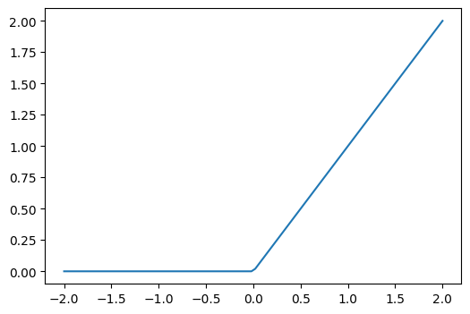
We finalize our neural net with torch definitions and train the model.
neural_net_example = torch.nn.Sequential(
    torch.nn.Linear(28 * 28, 30), torch.nn.ReLU(), torch.nn.Linear(30, 1)
)

opt = BasicOptim(neural_net_example.parameters(), lr=0.1)


train_model(neural_net_example, 20)
0.599 0.7904 0.888 0.9375 0.9552 0.9644 0.9709 0.9717 0.9704 0.9743 0.9743 0.9743 0.9756 0.9756 0.9769 0.9769 0.9795 0.9795 0.9795 0.9795
Note about scoping in the last snippet, does train_model pick up the latest definition of opt? train_epoch doesn’t take opt as an argument — instead, it references opt from the outer (global) scope.
When Python executes train_epoch, it looks up the name opt in that global scope.
When you reassign opt to a new optimizer object before calling train_model, that new object will be the one train_epoch sees when it runs.