recurrent neural net

Recurrent Neural Net (RNN) uses recursion as a strategy to create deep neural nets. By incorporating recursion, it allow nn to retain more information, giving them “memory” of longer sequences of information. RNNs use the same hidden weight matrix for all additional layers, which make it memory efficient. It trains this weight matrix by recursively incorporating the next token in the training sequence (like a sentence). RNN is best suited for sequential data like natural language or time series.

Suppose the hidden layer is $W$, $e$ are token embeddings, and $h_o$ is the output layer:

The first hidden state/activation is

$$h_0=\text{ReLU}(W{e}_0+b)$$

The second hidden state is

$$h_1=\text{ReLU}(W(h_0+e_1)+b)$$

The third hidden state:

$$h_2=\text{ReLU}(W(h_1+e_2)+b)$$

The output predictions:

$$\text{logits}=h_o(h_2)$$

Notice that throughout this process, the hidden layer, $W$, stays the same in the forward pass.

In general, the standard RNN is formulated as

$$h_t=f(W{h}_{t-1}+U{e}_t+b)$$

• $h_{t-1}$ : previous hidden state
• $e_t$ : embedding (input at this step)
• $W$ : hidden-to-hidden weights (processes the past)
• $U$ : input-to-hidden weights (processes the current token)
• $b$ : bias
• $f$ :the activation function

Data Preparation

# !wget "https://s3.amazonaws.com/fast-ai-sample/human_numbers.tgz" -O "../data/human_numbers.tgz" && tar -xzf "../data/human_numbers.tgz" -C ../data/
 

import torch
import torch.nn as nn
import torch.nn.functional as F
from torch.utils.data import DataLoader

from pathlib import Path
 
sample_path = Path("../data/human_numbers")
print(list(sample_path.iterdir()))

[PosixPath('../data/human_numbers/train.txt'), PosixPath('../data/human_numbers/valid.txt')]

lines = []
with open(sample_path / "train.txt") as f:
    lines += [*f.readlines()]
with open(sample_path / "valid.txt") as f:
    lines += [*f.readlines()]
len(lines)
 

9998

Our dataset consists of words of numbers and periods. We calculate the vocab size of this dataset:

text = " . ".join([l.strip() for l in lines])
tokens = text.split(" ")
vocab = set(tokens)
tokens[:10], len(vocab), list(vocab)[:10]

(['one', '.', 'two', '.', 'three', '.', 'four', '.', 'five', '.'],
 30,
 ['fifty',
  'eleven',
  'ninety',
  'five',
  'four',
  'eighteen',
  'sixty',
  'forty',
  'one',
  'seven'])

We convert tokens into index:

word2idx = {w: i for i, w in enumerate(vocab)}
nums = [word2idx[i] for i in tokens]
len(nums)

63095

We will predict every word given the previous words. Todo so, we define the sequence length as sl, each element in seqs now contains 2 element, offset by 1 index.

sl = 16
seqs = [
    (torch.tensor(nums[i : i + sl]), torch.tensor(nums[i + 1 : i + sl + 1]))
    for i in range(0, len(nums) - sl - 1, sl)
]
cut = int(len(seqs) * 0.8)
seqs[:5]

[(tensor([ 8, 20, 28, 20, 19, 20,  4, 20,  3, 20, 18, 20,  9, 20, 25, 20]),
  tensor([20, 28, 20, 19, 20,  4, 20,  3, 20, 18, 20,  9, 20, 25, 20, 10])),
 (tensor([10, 20, 22, 20,  1, 20, 11, 20, 29, 20, 21, 20, 13, 20, 16, 20]),
  tensor([20, 22, 20,  1, 20, 11, 20, 29, 20, 21, 20, 13, 20, 16, 20, 15])),
 (tensor([15, 20,  5, 20, 24, 20, 12, 20, 12,  8, 20, 12, 28, 20, 12, 19]),
  tensor([20,  5, 20, 24, 20, 12, 20, 12,  8, 20, 12, 28, 20, 12, 19, 20])),
 (tensor([20, 12,  4, 20, 12,  3, 20, 12, 18, 20, 12,  9, 20, 12, 25, 20]),
  tensor([12,  4, 20, 12,  3, 20, 12, 18, 20, 12,  9, 20, 12, 25, 20, 12])),
 (tensor([12, 10, 20, 14, 20, 14,  8, 20, 14, 28, 20, 14, 19, 20, 14,  4]),
  tensor([10, 20, 14, 20, 14,  8, 20, 14, 28, 20, 14, 19, 20, 14,  4, 20]))]

We also need a DataLoader to generate continuous sequences across batch in order so that the model can accumulate activations across batches. That’s to say, if we have batch size bs, our dataset is divided into m = len(dset) // bs groups (the # of batches). Across these groups, sequence at index i should follow one another. That is to say, ith sequence in every batch should follow one other.

For example, our sequences are defined for every 3 words:

[(tensor([2, 6, 5]), 6), (tensor([ 6, 16,  6]), 27), (tensor([27,  6, 29]), 6)]

Our batches should be structured to connect this sequence across batch (notice the 1st elem of each batch come from the sequence). In this case, we have 3 batches each of size 3:

(tensor([[ 2,  6,  5],
         [ 8, 14,  4],
         [29,  8, 27]]),
 tensor([[ 6, 16,  6],
         [25, 29,  6],
         [ 4, 25,  5]]),
 tensor([[27,  6, 29],
         [ 5,  8, 14],
         [ 6, 29,  8]]))

We define group_chunks to load our dataset based on the logic above.

def group_chunks(ds, bs):
    m = len(ds) // bs
    new_ds = []
    for i in range(m):
        new_ds += [ds[i + m * j] for j in range(bs)]
    return new_ds
 
bs = 64
dls_train = DataLoader(group_chunks(seqs[:cut], bs), batch_size=bs, drop_last=True)
dls_valid = DataLoader(group_chunks(seqs[cut:], bs), batch_size=bs, drop_last=True)

xb, yb = next(iter(dls_train))
xb.shape,yb.shape

(torch.Size([64, 16]), torch.Size([64, 16]))

RNN

We define a classic RNN below:

class LMModel4(nn.Module):
    def __init__(self, vocab_sz, n_hidden, bs):
        super().__init__()
        # input layer
        self.i_h = nn.Embedding(vocab_sz, n_hidden)
        # hidden layer
        self.h_h = nn.Linear(n_hidden, n_hidden)
        # output layer
        self.h_o = nn.Linear(n_hidden, vocab_sz)
        # store dimensions for proper initialization
        self.n_hidden = n_hidden
        # initiate hidden state properly
        self.h = torch.zeros(bs, n_hidden)
        # self.h = None
 
    def forward(self, x):
        _, sl = x.shape
 
        out = []
        for i in range(sl):
            # Add embedding to hidden state
            self.h = self.h + self.i_h(x[:, i])
            # Apply hidden layer with activation
            self.h = F.relu(self.h_h(self.h))
            # Generate output for this timestep
            out.append(self.h_o(self.h))
        
        # Detach hidden state to prevent gradient explosion
        self.h = self.h.detach()
        return torch.stack(out, dim=1)
 
    def reset(self):
        """Reset the hidden state"""
        self.h = torch.zeros(bs, self.n_hidden)
 

The output shape of the model is bs x sl x vocab_sz, our valid data are bs x sl

xb, yb = next(iter(dls_train))
rnn2 = LMModel4(len(vocab), 64, bs)
rnn2(xb).shape, xb.shape, yb.shape

(torch.Size([64, 16, 30]), torch.Size([64, 16]), torch.Size([64, 16]))

Our loss function need to be modified to align the dimensions:

print(rnn2(xb).view(-1, len(vocab)).shape, yb.view(-1).shape)
F.cross_entropy(rnn2(xb).view(-1, len(vocab)), yb.view(-1))
 

torch.Size([1024, 30]) torch.Size([1024])





tensor(3.4497, grad_fn=<NllLossBackward0>)

Based on the above, we define our loss function:

def loss_func(inp, targ):
    return F.cross_entropy(inp.view(-1, len(vocab)), targ.view(-1))

We also define batch accuracy for our training:

def batch_accuracy(pred, target):
    # pred: (bs, sl, vocab), targ: (bs, sl)
    return (pred.argmax(-1) == target).float().mean().item()
 

print(f"Training batches: {len(dls_train)}")
print(f"Validation batches: {len(dls_valid)}")

Training batches: 49
Validation batches: 12

We will write a standard training loop.

Notice that we reset the hidden state of the model at the beginning of each train and validation phases of an epoch by calling the reset method defined in the model. this will make sure we start with a clean state before reading those continuous chunks of text.

epochs = 20
# Use a lower learning rate to start
rnn2 = LMModel4(len(vocab), 64, bs)
 
optimizer = torch.optim.SGD(rnn2.parameters(), lr=0.01, momentum=0.9, weight_decay=5e-4)
scheduler = torch.optim.lr_scheduler.OneCycleLR(
    optimizer, max_lr=0.01, steps_per_epoch=len(dls_train), epochs=epochs
)
 
 
# torch.backends.cudnn.benchmark = True  # good if input sizes are consistent
def train(model, epochs, train_loader, valid_loader):
    for epoch in range(epochs):
        epoch_loss = torch.zeros(())
        batch_num = 0
        model.train()
        model.reset() # reset hidden state at the beginning of each epoch
        for xb, yb in train_loader:
            pred = model(xb)
            loss = loss_func(pred, yb)
            loss.backward()
            optimizer.step()
            scheduler.step()
            optimizer.zero_grad()
            epoch_loss += loss.item()
            batch_num += 1  # number of batches within a epoch
        avg_loss = epoch_loss / batch_num
        model.eval()
        model.reset()
        with torch.no_grad():
            batch_num_valid = 0
            valid_loss = 0
            valid_acc = 0
            for xb, yb in valid_loader:
                pred = model(xb)
                valid_loss += loss_func(pred, yb).item()
                valid_acc += batch_accuracy(pred, yb)
                batch_num_valid += 1
        print(f"epoch {epoch}, train loss: {avg_loss:.4f}")
        print(f"validation loss {valid_loss / batch_num_valid:.4f}")
        print(f"validation accuracy {valid_acc / batch_num_valid:.4f}")

train(rnn2, epochs, dls_train, dls_valid)

epoch 0, train loss: 3.3648
validation loss 3.2658
validation accuracy 0.1025


epoch 1, train loss: 2.8509
validation loss 2.6469
validation accuracy 0.2459
epoch 2, train loss: 2.0083
validation loss 2.0225
validation accuracy 0.4651
epoch 3, train loss: 1.5979
validation loss 1.9134
validation accuracy 0.4695
epoch 4, train loss: 1.5244
validation loss 1.8921
validation accuracy 0.4628
epoch 5, train loss: 1.4827
validation loss 1.8661
validation accuracy 0.4596
epoch 6, train loss: 1.4420
validation loss 1.8273
validation accuracy 0.4598
epoch 7, train loss: 1.4049
validation loss 1.8006
validation accuracy 0.4674
epoch 8, train loss: 1.3770
validation loss 1.7890
validation accuracy 0.4733
epoch 9, train loss: 1.3497
validation loss 1.7694
validation accuracy 0.4794
epoch 10, train loss: 1.3219
validation loss 1.7587
validation accuracy 0.4907
epoch 11, train loss: 1.2936
validation loss 1.7449
validation accuracy 0.5023
epoch 12, train loss: 1.2624
validation loss 1.7234
validation accuracy 0.5144
epoch 13, train loss: 1.2315
validation loss 1.7028
validation accuracy 0.5200
epoch 14, train loss: 1.2096
validation loss 1.7351
validation accuracy 0.5142
epoch 15, train loss: 1.1770
validation loss 1.7412
validation accuracy 0.5120
epoch 16, train loss: 1.1597
validation loss 1.7288
validation accuracy 0.5212
epoch 17, train loss: 1.1408
validation loss 1.7306
validation accuracy 0.5225
epoch 18, train loss: 1.1299
validation loss 1.7316
validation accuracy 0.5240
epoch 19, train loss: 1.1253
validation loss 1.7264
validation accuracy 0.5273

Long Short-Term Memory (LSTM)

One problem with RNN is vanishing/exploding gradients. Since a sequence is very long, while updating our hidden layer, we multiply gradients by many times, this can make gradients very small/large. Instead of using a simple nn as a hidden layer, we use four nn, so instead of

$$h_t=f(W{h}_{t-1}+U{e}_t+b)$$

We use a LSTM cell that include four neural nets (orange boxes), as shown below.

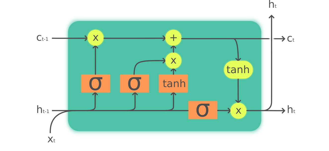
The LSTM cell includes two hidden states instead of one in classic RNN. In classic RNN, the hidden state is responsible for:

1. Having the right information for the output layer to predict the correct next token
2. Retaining memory of everything that happened in the sentence

It turns out that RNN is bad at memorizing things distant in the memory. So we introduces a cell state to keep track of the memory. The cell state is labeled $C$ in the figure. It is mainly responsible for keeping track of memory through selectively adding and forgetting things. The hidden state $h$ is responsible for sending things to the cell state thru nns and return output.

The four neural nets are named: forget gate (sigmoid), input gate (sigmoid), cell gate (tanh) and output gate (sigmoid). For detailed walk thru of LSTM, see Colah’s article linked below.

Now we create a literal translation based on the LSTM diagram above:

class LSTMCell(nn.Module):
    def __init__(self, ni, nh):
        self.forget_gate = nn.Linear(ni + nh, nh)
        self.input_gate  = nn.Linear(ni + nh, nh)
        self.cell_gate   = nn.Linear(ni + nh, nh)
        self.output_gate = nn.Linear(ni + nh, nh)
 
    def forward(self, input, state):
        h,c = state
        h = torch.cat([h, input], dim=1)
        forget = torch.sigmoid(self.forget_gate(h))
        c = c * forget
        inp = torch.sigmoid(self.input_gate(h))
        cell = torch.tanh(self.cell_gate(h))
        c = c + inp * cell
        out = torch.sigmoid(self.output_gate(h))
        h = out * torch.tanh(c)
        return h, (h,c)

We recreate the model using pytorch’s LSTM model:

class LMModel5(nn.Module):
    def __init__(self, vocab_sz, n_hidden, n_layers):
        super().__init__()
        self.i_h = nn.Embedding(vocab_sz, n_hidden)
        self.rnn = nn.LSTM(n_hidden, n_hidden, n_layers, batch_first=True)
        self.h_o = nn.Linear(n_hidden, vocab_sz)
        self.h = [torch.zeros(n_layers, bs, n_hidden) for _ in range(2)]
        
    def forward(self, x):
        res,h = self.rnn(self.i_h(x), self.h)
        self.h = [h_.detach() for h_ in h]
        return self.h_o(res)
    
    def reset(self): 
        for h in self.h: h.zero_()

We also train for 20 epochs. We also switched to AdamW optimizer for better performance since there are significantly more layers to train. As we can see, the accuracy is higher with LSTM.

epochs = 20
rnn3 = LMModel5(len(vocab), 64, 2)
optimizer = torch.optim.AdamW(rnn3.parameters(), lr=3e-3, weight_decay=1e-2)
scheduler = torch.optim.lr_scheduler.OneCycleLR(
    optimizer, max_lr=3e-3, steps_per_epoch=len(dls_train), epochs=epochs
)
 
train(rnn3, epochs, dls_train, dls_valid)

epoch 0, train loss: 3.3625
validation loss 3.3053
validation accuracy 0.1511
epoch 1, train loss: 2.8902
validation loss 2.7392
validation accuracy 0.3241
epoch 2, train loss: 2.2055
validation loss 1.8999
validation accuracy 0.4600
epoch 3, train loss: 1.5229
validation loss 1.8163
validation accuracy 0.4513
epoch 4, train loss: 1.3620
validation loss 1.8125
validation accuracy 0.4869
epoch 5, train loss: 1.2466
validation loss 2.0368
validation accuracy 0.4884
epoch 6, train loss: 1.1412
validation loss 2.1412
validation accuracy 0.5374
epoch 7, train loss: 1.0477
validation loss 2.1705
validation accuracy 0.5298
epoch 8, train loss: 0.9251
validation loss 2.1211
validation accuracy 0.5409
epoch 9, train loss: 0.8050
validation loss 1.8328
validation accuracy 0.5688
epoch 10, train loss: 0.6615
validation loss 1.9828
validation accuracy 0.5781
epoch 11, train loss: 0.5230
validation loss 1.8785
validation accuracy 0.6050
epoch 12, train loss: 0.4152
validation loss 1.9530
validation accuracy 0.6322
epoch 13, train loss: 0.3382
validation loss 1.9337
validation accuracy 0.6369
epoch 14, train loss: 0.2831
validation loss 1.9904
validation accuracy 0.6559
epoch 15, train loss: 0.2449
validation loss 1.9130
validation accuracy 0.6693
epoch 16, train loss: 0.2235
validation loss 1.9406
validation accuracy 0.6796
epoch 17, train loss: 0.2107
validation loss 1.9669
validation accuracy 0.6746
epoch 18, train loss: 0.2050
validation loss 1.9519
validation accuracy 0.6758
epoch 19, train loss: 0.2033
validation loss 1.9550
validation accuracy 0.6753

References

1. Colah, Understanding LSTM Networks: https://colah.github.io/posts/2015-08-Understanding-LSTMs/